Overview

Our team built and tested an integrated cleaning and inspecting pig (ICIP). We implemented this as a short-bodied mandrel pig outfitted with inexpensive sensors. Our motivating use case is monitoring internal erosion and pitting in small-diameter flow lines.

ICIPs are ideal for monitoring rapid time-scale events because small crews can deploy them quickly using pigging valves. Because they are based on cleaning pigs, they can traverse pipelines that larger-bodied inspecting pigs cannot. An operator would deploy a sequence of ICIPs to scan the pipe when they suspect it is under an active threat.

The first installment of this write-up, which can be found here, described the selection of sensors, the circuitry design, and the pig’s construction. This second installment evaluates how well inexpensive proximity sensors can “see” the inside of a pipe.

The contents of this post are:

1. Overview
2. Results
   1. Notes
3. Objective: Sensor characterization
4. Testing Setup
   1. Sensors
   2. Test track and cart
   3. Test plates
5. Sensor Parameters
   1. Standoff Distance
   2. Inter-sensor spacing
   3. Sampling
   4. Submersion tests
   5. Angle of incidence testing
   6. Embedding test
6. Testing Results
   1. Results for plate one
   2. Results for plate two
      1. End Notes

Results

We used commercially available proximity sensors, the Long Range Inductive Proximity Sensor X0036 by Fargo Controls, with an operating range of 36 mm (1.4 in). This sensor was able to resolve a 6.4 mm (0.25 in) diameter flat-bottomed hole that was 2.4 mm (0.09 in) deep at a standoff distance of 5.46 mm (0.215 in). This distance is 15% of the sensor’s published operating range.

A longer-range version of this sensor is available with a range of 150 mm (5.9 in). If the relationship between the sensor’s operating range and resolution threshold is linear, this more expensive sensor should support a standoff distance of 26.8 mm (1.06 in). Here, we evaluate the less expensive sensor as a proxy for the longer-range version.

For the tested sensors, we found a standoff distance of 5.46 mm (0.215 in). Since there appears to be little interference between adjacent sensors, we were able to deploy them with a center-to-center distance equal to the sensor diameter.

We calculate the axial resolution as a function of pig velocity, scan rate, and an agreement threshold of three readings. The tested sensors can see a 10 mm defect when moving at 1.7 m/s at a sample rate of 500 Hz.

We also explored three of the sensor’s ancillary properties that would predict their ability to operate in dirty pipes with tight bends. We found that the sensing signal was not noticeably affected by oily dirt in the interstitial space between the sensor and the test plates. To evaluate the sensor’s ability to navigate bends, the sensors were able to generate meaningful signals at angles up to 30 degrees from the plate surface. Finally, to demonstrate the ability to embed the sensors in the pig’s urethane drive cups, we demonstrated no noticeable signal attenuation from embedded sensors.

Notes

This is the second post in a two-part series about our team of undergraduate engineering students at the Colorado School of Mines’ two-semester, multidisciplinary capstone project. These projects allow the students to apply what they have learned in their studies to a real project. I was the sponsor and project mentor. The project presented here won the best-in-show Senior Capstone Design award.

This is my write-up using the data the team collected per my specifications.

All images in this document link to higher-resolution versions. Click on an image to enlarge it.

Objective: Sensor characterization

Tests were designed to understand the following fundamental properties of these sensors:

• Sensor standoff distance
  • How is the sensor signal affected by distance from the pipe wall?
  • What is the optimal distance for this sensor?

• Inter-sensor spacing
  • How much between-sensor spacing is required to avoid interference?
  • What is the best radial resolution using side-by-side sensors?
• Sampling
  • How quickly can the sensors and circuitry take measurements?
  • What is the best axial resolution as a function of velocity and sample rate?
  • What is the expected battery life of this pig?

We also did some testing to understand these important ancillary properties:

• Sensor obstruction
  • How do pipe wall deposits affect sensor readings?
  • How do pipe fluids affect sensor readings?
• Sensing angle
  • How are readings affected as the pig traverses a bend?
  • How are readings affected by mechanical damage to the pig or pipe wall?
• Embedding
  • Can the sensors be embedded in the drive disks?

Testing Setup

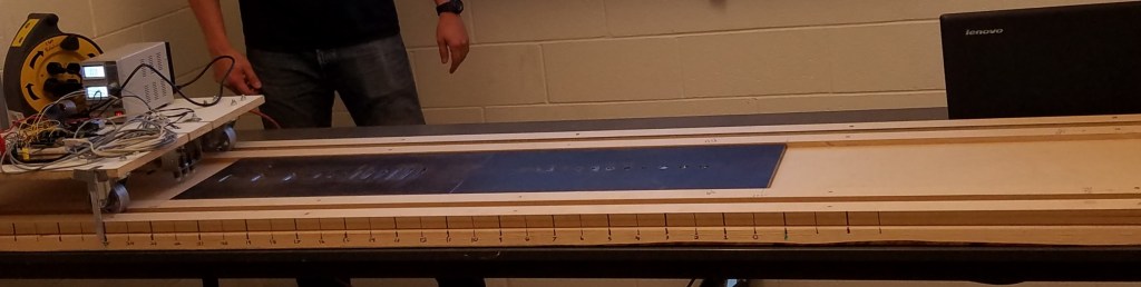
The testing apparatus consisted of a cart and a test track. The cart held the sensors and electronics. The test track consisted of two steel plates with 24 artificial defects. Three sensors were mounted perpendicular to the direction of the cart’s travel along the track. This is shown in Figure 01.

Each of these elements is described in the sections that follow.

Testing involved rolling the cart along the track. As the cart moves, the electronics record a voltage signal from the sensors. These sensor voltages correspond to the distance between the sensor tip and the steel target. Voltage readings are sampled and stored according to the process described in part one.

To simulate the variable velocity experienced by pigs, the cart was moved by hand. The instantaneous speed at each timestep was measured by video on the horizontal scale.

Sensors

Inductive proximity sensors use an inductive coil and an oscillator within the sensor to create an electromagnetic field around the sensor’s tip. When a metallic object comes within sensing distance, the magnetic field is disrupted, and the oscillations are dampened. A threshold circuit identifies the changes in the oscillations and outputs voltages proportional to the distance from the metal target.

The design use case for these sensors is detecting the presence or absence of a chunk of metal within the operating distance. In contrast, our use case was to measure the distance to the metal. When there is internal metal loss, the pipe wall is further away.

The sensors we used, the Long Range Inductive Proximity Sensor X0036 by Fargo Controls, were 12 mm (0.47 in) in diameter and had an operating range of 36 mm (1.4 in). The current draw is less than 8 mA, operating at frequencies between 100 and 500 Hz. Distance to the pipe wall is seen as a voltage drop, where zero distance is at the voltage minimum, and infinite distance is the baseline voltage.

We found the sensors could resolve defects as small as 0.1 \textrm{\ in} at about fifteen percent of the published operating distance. At around 18\% of the operating range, the signal becomes noisy. The signal-to-noise ratio beyond this distance is too low to resolve the smallest features.

Some sensors in this product line have a much larger operating range of 150 mm (5.9 in). Fifteen percent of this working range is 23.1 mm (0.91 in), and eighteen percent is 26.8 mm (1.1 in).

Test track and cart

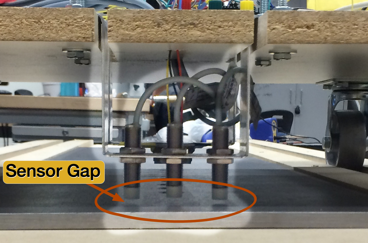
Three sensors are mounted to the underside of the cart on an adjustable bracket. This bracket allowed us to adjust:

• the spacing between the sensors,
• the standoff height between the sensors and the test plates, and
• the angle of incidence between the sensors and the plates.

The standoff distance, which is the gap between the sensor tip and the average surface of the plate, is shown in Figure 02.

Test plates

Figure 03 is a mechanical drawing of the two steel test plates. Each plate was 24 inches long by 12 inches wide by 3/8-inch thick. These two plates contained 24 target defects of various geometries: cylindrical holes, radial slots, and equilateral triangles.

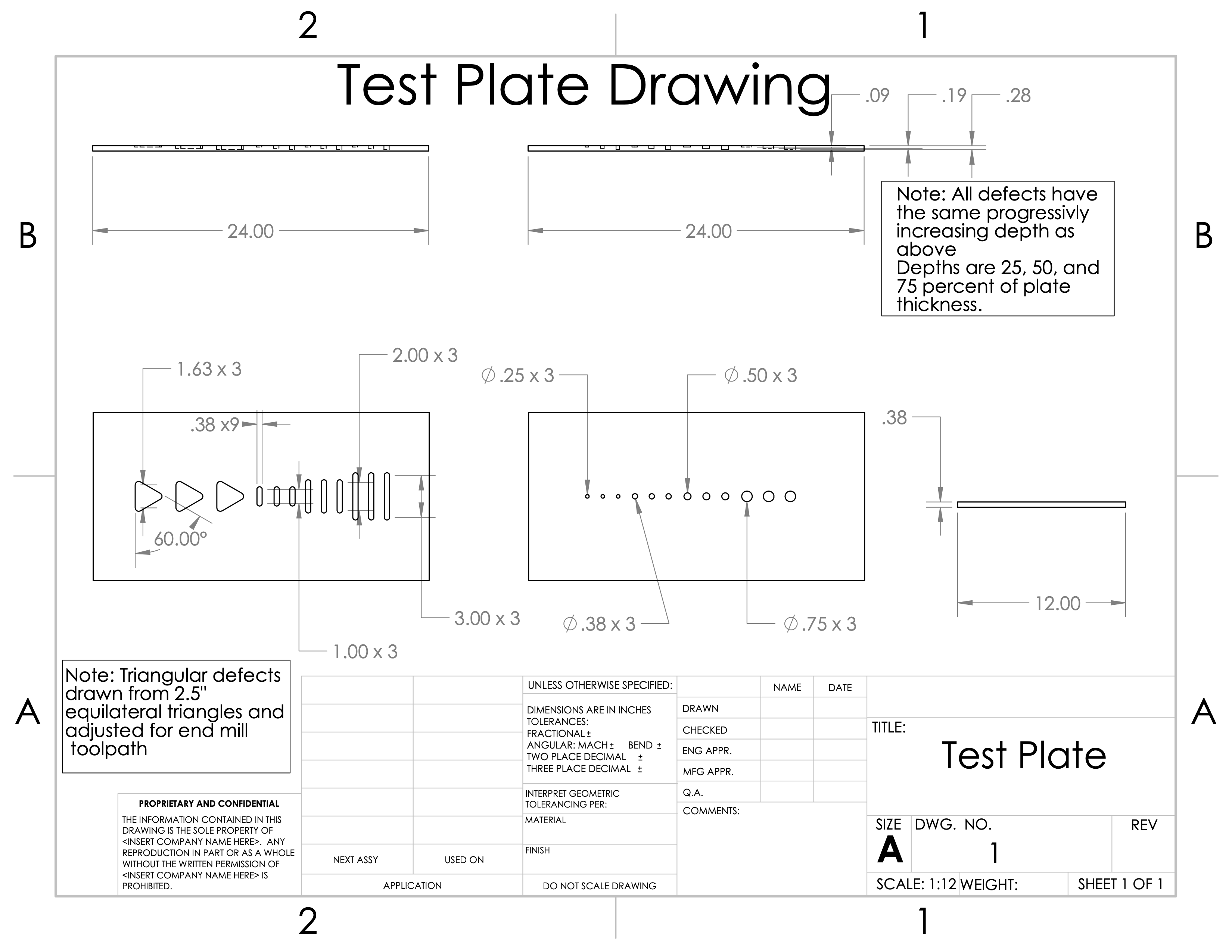
Each target geometry was machined to 25%, 50%, and 75% of the wall thickness. For the 9.5 mm (3/8 in) plates, these depths are 2.4 mm (0.09 in), 4.8 mm (0.19 in), and 7.1 mm (0.28 in). The targets were arranged axially in groups of three, one target of each shape at each of these depths.

Figure 03 shows the size and positioning of the defects. Figure 04 is a photo of the test plates showing how targets are grouped in threes by target depth.

Plate One contained 12 flat-bottomed cylindrical holes arranged axially in a line down the center of the plate. This arrangement was designed to test the ability of the sensors to “see” only the section of pipe directly underneath them. In an ideal case, the center sensor would see the test holes, and the two adjacent sensors would see nothing.

Recall that the sensors were 12 mm (0.47 in) in diameter. The smaller target holes were 9.5 mm (1/4 in) and 6.4 mm (3/8 in). If the sensing area is constrained to the space under the sensor, the center sensor should see these smaller holes, and the left and right sensors should see nothing.

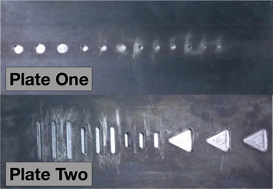
The larger holes were 13 mm (1/2 in) and 19 mm (3/4 in). The 13 mm hole is very similar to the 12 mm diameter of the sensor. The left and right sensors are expected not to detect this hole size. The 19 mm hole is substantially larger than the sensor diameter. When traversing this largest hole size, the left and right sensors should see a small signal.

Plate Two contained slots and triangles. Slots were arranged in one-inch increments from one to three inches long. There were nine slots in total, one slot for each depth. These nine slots were followed by three 2.5-inch equilateral triangles, one at each depth. This arrangement tested the ability of the sensors to work together to report the shape of a defect.

Sensor Parameters

This section presents our findings on the six key parameters we investigated for these sensors.

First, this section reports the best settings for the primary sensor properties: sensor standoff height, radial spacing, and sample rate. Next, it investigates the ancillary properties: the ability to function when dirty, sensing angle, and the ability to be embedded in the pig’s urethane drive disks.

Standoff Distance

The standoff distance is the distance between the sensors and the pipe wall. A larger standoff distance allows the pig to handle dirty pipe walls, which is a critical concern for the target use case of this tool. Figure 05 from McNealy 2024 shows cleaning pigs from pipelines that are difficult to inspect because they are difficult to clean.

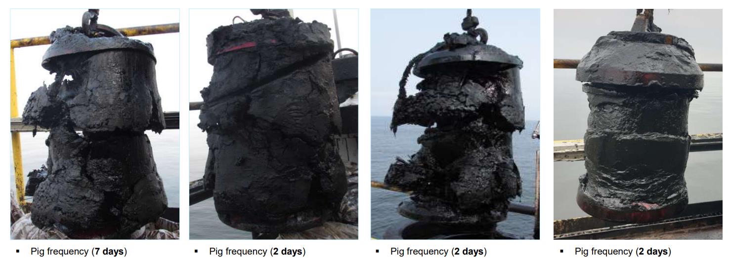
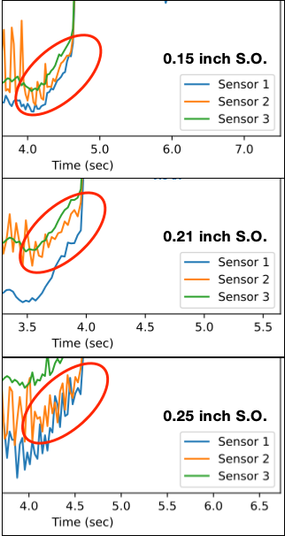
Figure 06 shows the impact of standoff distance on the sensor signal. These three graph segments show the three smallest holes on on Plate One. The red oval in each plot indicates where we expect to see three spikes, one for each of the three quarter inch diameter holes.

The top graph was taken with a standoff (“S.O.”) of 3.8 mm (0.15 in). This is 11% of the sensor’s published operating range of 36 mm (1.4 in). The center graph was recorded at a standoff of 5.3 mm (0.21 in), 15% of the sensor’s published operating range. The bottom graph was recorded with a standoff of 6.4 mm (0.25 in), 18% of the sensor’s published operating range.

These defects are clear in the smallest standoff graph at the top. In contrast, the noise is approximately the same magnitude as the signal in the largest standoff graph at the bottom. This larger standoff makes it more difficult to see these small holes.

This figure shows how the signal-to-noise ratio decreases with increasing standoff distance. The signal for the smallest standoff distance follows the topography of the manufactured defects in each plate. The signal for the largest standoff distance is much noisier.

Based on these results, we used a standoff distance of 5.46 mm (0.215 in) for all subsequent testing.

Inter-sensor spacing

The spacing between sensors determines the radial resolution.

Sensors are arranged circumferentially in a ring around an inspecting pig’s perimeter. The center-to-center distance between adjacent sensors is the radial resolution. This distance is determined by the sensor’s physical dimensions and any physical separation necessary to prevent adjacent sensors from interfering. This is experienced as the number of scan lines in an inspection’s signal graph. There is one scan line for each sensor.

The proximity sensors used here are active. They generate a baseline inductive field. The signal we read is a disturbance in this field. It is plausible that if we place these sensors too close together, the adjacent inductive fields could interfere, invalidating the readings.

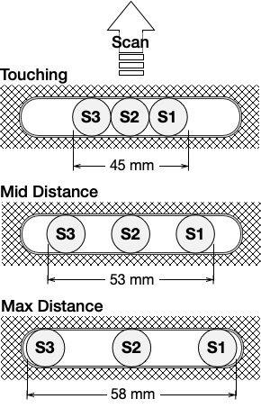
Figure 07 shows the radial spacing configurations that we tried. We incrementally reduced the spacing from the Max Distance to Touching. We observed that when the sensors were physically touching, and we ran them across the slot patterns and triangles on Plate two, there was only a signal when the sensor was directly over a defect. This indicates that there is minimal interference when the sensors are touching.

Since touching sensors is the best possible resolution in a single ring, all subsequent testing was done with the sensors in the Touching configuration.

Sampling

Sampling behavior dictates the velocity-dependent axial resolution of the pig. Also, the sampling strategy affects battery life, memory consumption, and answer precision.

The sensors we used had a published sample rate of 500 Hz. The more capable sensors, with the larger sensing distance, were limited to 100 Hz. The company offers other sizes that operate at sample rates of 400 Hz and 500 Hz. Higher sample rates use more battery and more memory. Both affect the tradeoff between the pig’s size and its operating range.

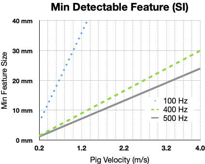
The axial resolution is the smallest feature that the pig can see in the length direction. Sample frequency and pig velocity combine to determine this resolution. This is shown in the graph of Figure 08, where the minimum detectable defect size is plotted against pig velocity for several representative sample rates.

Since faster sample rates take more sample points over each unit of distance, faster sample rates resolve smaller features. Now, holding the sample rate constant, the distance between each sample point increases when the pig moves faster and decreases when the pig slows down. So, slow pigs with fast sample rates can see the smallest features.

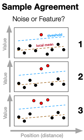
While the sample rate and pig velocity determine the smallest feature that can reliably be sensed with a single sample point, this is not enough information to identify what the pig can “see”. Figure 09 demonstrates that to see a feature, it must be recognized as being outside the local mean signal value and not noise.

We can set a threshold based on the local mean error function to recognize a sample point outside the local mean signal value. This threshold is the upper dashed line that follows the slope of the local mean in Figure 09. Features that generate a signal with a value less than this threshold cannot be detected.

As shown in Figure 09, a solitary reading outside the threshold may represent a small feature, or it may be noise. If there are two consecutive samples with similar values, they may represent a feature, or they may also be noise. After some number of features with similar values outside the threshold, one can have confidence that these locally aberrant signals agree that there IS a feature at this location.

This need for sample point agreement increases the minimum detectable feature size by requiring some minimum number of sample points in agreement to declare that there is a feature. The graph in Figure 08 was created by requiring three sample points.

Submersion tests

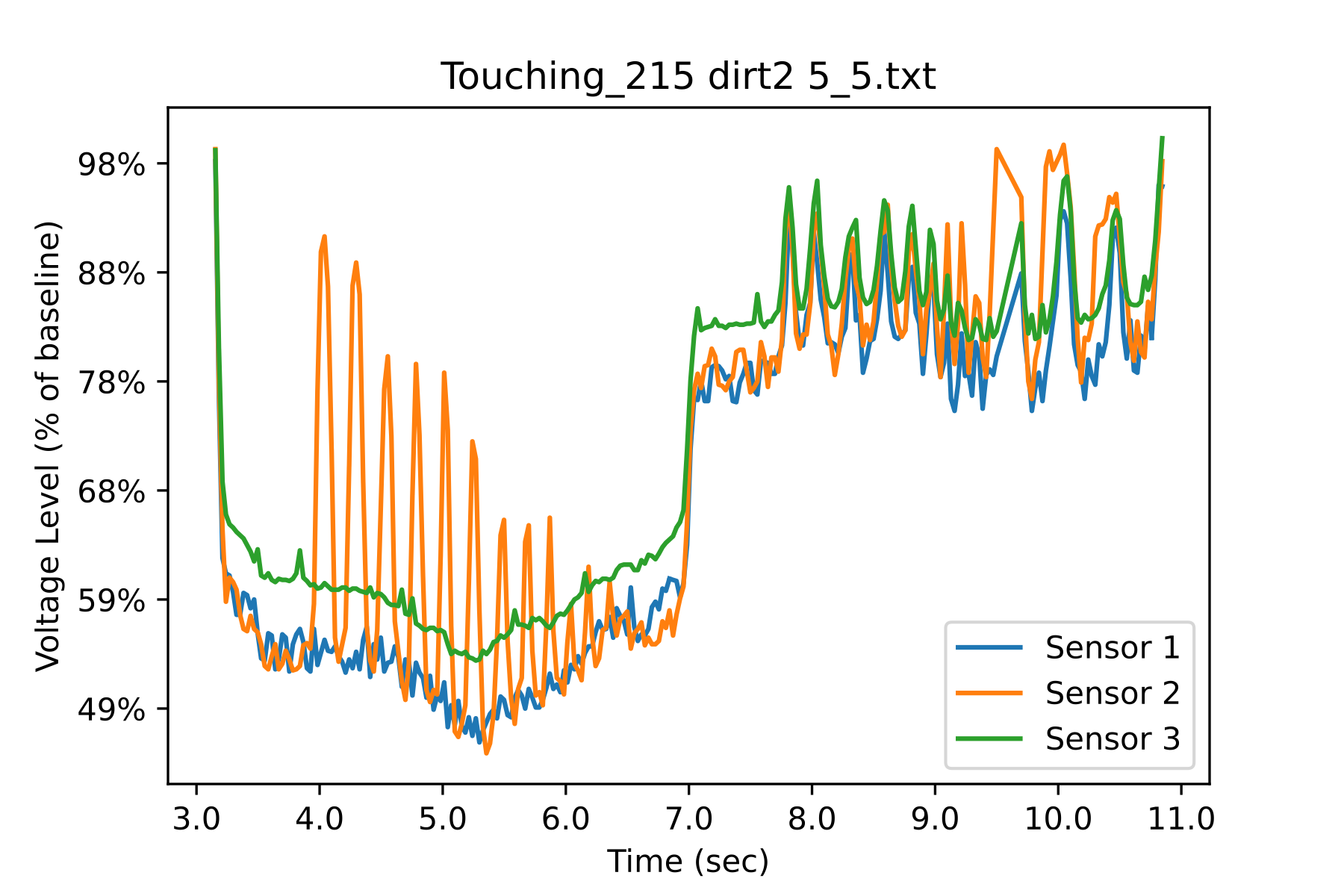
We tested the sensors’ performance when submerged in water, oil, or oily dirt. Figure 10 shows the sensor trace for the oily dirt. Here, the baseline is noisier because the sensors were moved very slowly, more than twice as slowly as in Figures 05 and 06. However, the results are functionally identical to those from the clean plates.

Angle of incidence testing

The angle of incidence captures the sensors’ ability to take meaningful readings while negotiating curves. We tested this by setting the horizontal spacing so the sensors were touching. The vertical standoff distance was set to 0.21 inches. We then ran a series of tests, increasing the sensors’ angle of incidence in small increments from vertical.

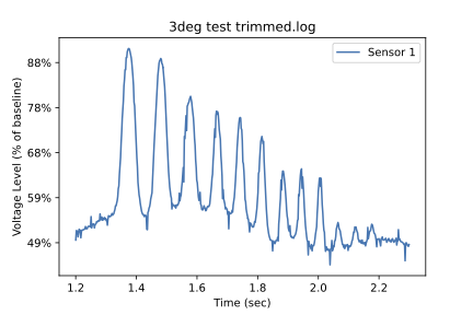
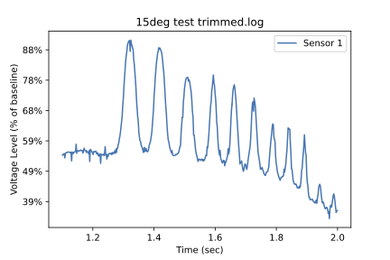
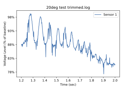
Figure 11 shows three graphs at sensor angles: 3, 15, and 20 degrees from vertical in the axial direction. This set of graphs shows that the relative amplitude at an angle of 3 degrees is about 40%, while it is only 10% at an angle of 20 degrees.

With a constant standoff, increasing the angle to 20 degrees reduces the relative amplitude by 30%. Since the signal is still useful at this angle, the pig should be able to take readings around most bends.

Embedding test

The mechanical design called for the sensors to be embedded in the urethane matrix of the pig’s disks. We chose a urethane density of 1060 kg/m^3 which, according to our FEA, gave us a balance of the rigidity necessary to support the pig and the compliance necessary to navigate pipe bends.

The urethane was transparent to the sensor signal. It caused no noticeable signal degradation, meaning this urethane could be used for the sensor disks. Because of this signal transparency, the primary impact of the urethane on the sensing is on the standoff distance.

Testing Results

Figure 12 shows a traverse of Plate One. Figure 13 is a traverse of Plate Two.

These data were collected with the following parameters:

• Standoff height (15% of range): 0.21 inches (5.3 mm) – plate to sensor tip
• Inter-sensor spacing: 0 inches (0 mm) – touching
• Center-to-center distance between sensors: 0.47 in (12 mm)
• Sample rate: 500 Hz

These graphs show one trace for each of the three sensors. The x-axis of these graphs is in time units of seconds. The y-axes show voltage. Each set of traces is scaled to the plate boundaries.

Both graphs include a scaled image of the test pattern. The 24 defect targets are numbered at the beginning of each group of three. Targets 1 to 12 are on Plate One. Targets 13 to 24 are on Plate Two.

Each numbered target has a dashed line that extends from the target geometry to the corresponding location on the voltage graph. The locations of unnumbered targets may be inferred by counting.

To the left of the target graphic is a set of three blue circles, which indicate the approximate arrangement of the three sensors as they traversed the plate. The middle Induction sensor was aligned at the centerline of the two test patterns. The scan proceeded axially along the indicated direction.

Results for plate one

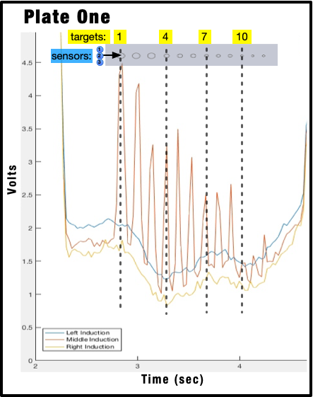
Figure 12 shows the result for test Plate One at the above settings. There are three key results for using these proximity sensors to measure metal loss in pit-like defects.

1. Sensors do not interfere with each other. Each seems to detect only the area of the target plate directly beneath itself.
2. For “defects” that are the same diameter as the sensor or larger, the voltage spike reflects the defect’s depth.
3. For “defects” smaller than the sensor diameter, the voltage spike reflects the defect’s diameter.

The spikes in the Middle Induction sensor curve correspond to the target holes.

There are no spikes on the Left or Right sensor curves. They are not noticeably affected by any of the center holes, even the targets larger than the sensor diameter. This suggests the sensors have a sensing pattern close to the sensor diameter. They do not overlap; they see only what is directly beneath them.

The voltage spike for Target 1 is about 2.75 volts high, the spike for Target 2 is about 2.5 volts, and Target 3 is only 2 volts high. This range is about 0.75 volts over these 3/4-inch (19 mm) diameter holes, which suggests that these three spikes show the decreasing depths of each target.

This difference in voltage spike size is less pronounced for the second group of targets, which are 1/2 inch (12 mm) in diameter. These targets, 4 to 6, are the same diameter as the sensor. The spike for Target 4 is about 2.25 volts high, and Target 6’s is 1.75 volts. The range over this group of three is 0.5 volts, which is two-thirds of the range of the first group.

This pattern of the voltage drop tracking the depth disappears by the third group. Targets 7 to 9 are 3/8 inch (9.5 mm) in diameter. This is smaller than the sensor diameter. Coincidentally, the voltage drop at the middle sensor for all three targets in this group is about 1 1/8 volts. The range of voltage drops over this group is zero since they are all the same.

This pattern continues for the fourth group of circular targets. The voltage spike for targets 10 to 12, which are all 1/4 inch (6 mm) in diameter, is only about 0.25 volts. This is similar to the noise level, meaning that this hole diameter is near the lower detection threshold for these sensors.

To summarize: The voltage spikes for defects 1-6, which are greater than or equal to the sensor diameter, correspond to the hole depth. The voltage spikes for defects 7-12 do not show this depth correspondence. However, the voltage spikes for these defects do seem to correlate to hole diameter.

Results for plate two

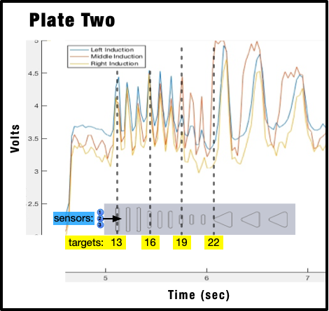
Figure 13 shows the result for test Plate Two at the above settings. There are three key results for using these proximity sensors to measure metal loss in larger defects.

1. For slots and triangles, the signal seems to be a function of depth whenever the sensor’s diameter is completely within the target.
2. The axial dimension of the slots being less than the sensor diameter introduces some complexity that should be examined further.
3. This arrangement of side-by-side sensors can discern the shape of defects from their voltage signal.

The three side-by-side sensors are about 1.5 inches (36 mm) wide along the radial axis. Compare this to the size of the slots, which are targets 13 to 21.

The largest slots, 13 to 15, are 3 inches (76 mm) wide in the radial direction. Since this is wider than the sensors, all three sensors “see” a strip of target that is at least as wide as they are. The voltage spikes for each of these slots decrease with slot depth. This is consistent with what was observed on test plate one.

The middle set of slots, targets 16 to 18, are 2 inches wide, which is still wider than the three sensors. Interestingly, the voltage spikes for this set are roughly the same as those for targets 13 to 15 in the first set of targets. Both sets yield a smaller signal as the target depth decreases.

This observation seems to support the previous section’s first result: that when a defect is larger than a sensor, the associated signal reflects the defect’s depth.

This relationship holds in the radial direction but not the axial one. Axially, each slot is only 0.38 inches (9.7 mm) long. The sensors are 0.47 inches (12 mm) in diameter. Despite the sensor being larger than the defect length, the signal decreases with the depth.

The third group of slots, targets 19 to 21, are only 1 inch wide. One would expect a reduction in signal with depth for the center sensor but not for the left and right sensors.

This is not exactly what happened. The center signal for target 19 is 1 volt tall, but the signals for targets 20 and 21 are about 0.8 volts tall. So, these center signals do not behave exactly as predicted. Still, the signals for the left and right sensors are about 1/3 volts for all three slot depths in this set, which matches the expectation.

Consider now the signals from the three equilateral triangle targets, which are 2.5 inches (64 mm) on a side. Because these targets are so large relative to the sensor size, voltage signal differences due to the depth are visible for all sensor traces in this set. Further, the shape of these targets can be inferred for each set by noticing that the signal for the left and right sensors rise only when these sensors pass directly over the target.

End Notes

1. R. Mcnealy, V. Ebrahimipour, D. Mendoza, and P. Kumar, Integrity Management of Difficult to “Smart-Pig” Pipelines Using Minimally Intrusive Sensors, Proceedings of the 36th Pipeline Pigging & Integrity Management Conference, 1-12, 2024. ↩︎

(c) Copyright 2025: Craig L. Champlin – Golden Colorado. All rights reserved.