Why can’t I use odometry for ILI runcoms?

- 15-minute read - written in simple language
- mildly technical, some simple math, BS in engineering

Introduction

Why is it so hard to match odometry readings?

Odometry is the in-pipe distance that an inline inspection tool has traveled since the start of the inspection. It serves as a distance-based index into the inspection data.

Odometry is understood to be a relative value that is useful for sorting inspection features but is otherwise useless for directly comparing them[1].

The disagreement between the odometry readings of two or more inline inspections can be many times larger than the length of a typical pipe spool. These errors accumulate rapidly. Over distances as short as 1.2 miles (2 km), the error can be too large to make useful comparisons[2]. The error accumulates unpredictably and nonlinearly. Plots of the relative error function between two inspections show random reversals, sharp perturbations, and other severe nonlinear behavior[3].

Over the years, there have been tremendous improvements in pipeline inspection technology. Many of these improvements appear aimed at solving the odometry problem. Vendors have outfitted pigs with multiple wheels. They have combined these wheels with onboard gyroscopes and accelerometers. Some pigs use no wheels, relying exclusively instead on inertial measurement units (IMUs) of various precisions. They have developed fancy algorithms to combine the inputs from all these sensors[4].

Still, odometry matching remains a problem. Why haven’t things improved?

This article presents an alternative to the common “wheel slip” model, which is the typical explanation for why odometry readings disagree.

This new model explains odometry errors as an inevitable consequence of the bias introduced during navigation by dead reckoning. The error from these dead-reckoning estimates accumulates during frequent updates to the onboard state machines, which estimate pig position (and accumulate bias) many times a second.

The model presented here explains why odometry sometimes overreports inspection length. It also explains why odometry can only be consistent when the exact same tool is used. Further, this model explains why odometry error is non-linear and, at times, erratic.

(Note: Text continues after the section references.)

K. Reber, M. Beller, and A. O. Barbian, Run Comparisons: Using in-line Inspection Data for the Assessment of Pipelines. Pipeline Technology Conference 2006, Proceedings (ISSN 2510-6716), 2006. ↩︎
Rosen. rocorr MFl-c service. Online, 2015. ↩︎
C. L. Champlin, Using odometry drift to match ILI joint boundaries for run comparisons, International Journal of Pressure Vessels and Pipelines, Vol. 213, 2025. ↩︎
Q. Ma, G. Tian, Y. Zeng, R. Li, H. Song, Z. Wang, B. Gao, and K. Zeng, Pipeline In-Line Inspection Method, Instrumentation and Data Management, Sensors, Vol. 21, , 2021. ↩︎

Measuring big things

Pipelines are big things. They must be measured by summing a sequence of smaller measurements.

Consider what it would take to measure a 100-yard American football field with a 10-foot tape measure. This would require at least 300 individual measurements. These smaller measurements would be combined into a chain of measurements that cover the larger distance.

Consider the mechanics of how you would do this.

You would likely begin by locking the tape at its longest length. If you don’t get the length exactly right, however, you introduce measurement bias that will be multiplied by 300. If you are off by only 1/16 inch, you will see a bias error of half a yard in your final measurement.

Next, you must decide how to connect adjacent measurements. The way you do this introduces additional systematic bias. Suppose you decide to drive a half-inch diameter stake into the ground to mark the end of each small measurement. Depending on how you use the stake, the stake diameter could increase or decrease your combined measurement by about four yards.

These measurement errors are significant and real. By the end of the measurement in this example, you are off by 4.5 yards. Yard lines on an American football field are spaced at 5-yard intervals. With rounding, your measurement error is an entire yard line!

As the length of a big thing increases, it becomes increasingly difficult to compare chained measurements.

Modeling a single measurement

Recall that all single measurements are random variables. These variables can be represented as a sum of their random and constant parts. Here, for distance measurements, we will break out the true length, bias, and random components.

Odometry is an estimate of position at some inspection feature. Position is a distance measure. Let the feature of interest, for example, the downstream end of the first pipe spool in a segment, be represented by the point labeled as $q$ . The single measurement at $q$ may be modeled as

Equation 1: $P_{q} = x_{q,\mathit{true}} + E_q + x_{q,\mathit{bias}}$

where the position estimate $P_q$ is a linear combination of the true position, $x_{q,\mathit{true}}$ , a zero-mean normally distributed random error term, $E_q$ , and a bias term, $x_{q,\mathit{bias}}$ .

Examining each term:

The true position $x_{q,\mathit{true}}$ is unknowable without lots of trials or some external information. It is a constant value but random error and the bias hide the true length.
The random error $E_q$ represents all sources of randomness in the measurement. It is modeled as a zero-mean normal distribution with some variance $E_q \sim (0, \sigma^2)$ .
The bias $x_{q,\mathit{bias}}$ represents all sources of systematic error in the measurement. It is a function of the tool and the technique. This is the quantity of interest for this article.

Equation 1 applies to a single measurement.

Combining measurements to measure big things

Combining measurements means adding individual measurements together in a summation. The technique by which individual measurements are combined introduces additional bias and error for each measurement. This additional bias and random error can be added to the existing bias and error terms of Equation 1.

Repeating Equation 1 in a summation over $N$ individual measurements will find the chained position measurement $P_N$ . This looks like:

Equation 2: $P_{N} = \sum\limits_{k=1}^N (\delta x_{k,\mathit{true}} + \delta x_{k,\mathit{bias}}) + \sum\limits_{k=1}^{N-1} E_k + E_N.$

This may look different, but it is just Equation 1 added together many times, once for each of the $N$ measurements. The $\delta$ in front of the true and bias terms, $\delta x_{k,\mathit{true}}$ and $\delta x_{k,\mathit{bias}}$ , indicate that these are for each individual sub measurement in the chain. Additionally, because the random error terms have a zero mean, they will cancel to zero since

Equation 3: $\lim_{N \rightarrow \infty}\left(\textrm{Exp}\left[\sum\limits_{k=1}^{N-1} E_k\right] \right) = 0.$

Finally, since the last individual measurement has randomness, there needs to be at least one random error term. This is the single $E_N$ at the end of Equation 2.

Equation 2 shows that although the random error cancels out, any bias in the individual measurements will accumulate when multiple measurements are combined. The more measurements there are in a measurement chain, the more significant the impact of the accumulated bias.

If you glazed over during this math talk, read the preceding paragraph and then skim through the example in the next section.

A toy example using ILI odometry

**Figure 1:** At the start of an inspection, x(0), the tool position is known exactly. For each subsequent estimate, there is measurement uncertainty, which is represented by the gray cloud around the tool at known locations x(1) and x(2). Within this uncertainty, a small amount of tool-specific measurement bias is represented by the cross-hatched patterns. This bias accumulates from one measurement to the next, shifting the mean value of the position estimate as it does so.

This example demonstrates the significant impact that bias has on position estimates. The measurement bias is what affects the odometry. The next section speculates on where this bias comes from.

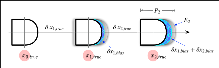
The position calculation of Equation 2 is illustrated in Figure 1, which shows a pig in three locations, $x_{0,\textit{true}}$ , $x_{1,\textit{true}}$ , and $x_{2,\textit{true}}$ . Pretend that these locations are girth welds, which are easy to identify in the inspection. In this way, the true location of the pig is known. What is unknown at each location is the reported odometry value.

The odometry value for the third location is labeled as the range $P_2$ . The odometry reading at the third girth weld is somewhere within this range. (It is a random value.) This position estimate is

Equation 4: $P_{2} = (\delta {x}_{1,\mathit{true}} + \delta {x}_{2,\mathit{true}}) + (x_{1,\mathit{bias}} + x_{2,\mathit{bias}}) + E_2$

which is simply a substitution of the variables from Figure 1 into Equation 2. We sum the two individual true distances, the two individual biases, and the one random error term. If there were more intermediate points, these would have also been added in.

Here, in this example, the cumulative bias, $\delta x_{1,\textit{bias}} + \delta x_{2,\textit{bias}}$ , is shown such that it overstates the odometry value. It is just as likely to understate it by being negative.

The random error term $E_2$ is shown as the gray cloud. When inspection vendors improve the reporting precision of a tool, they reduce this random error term. This model explains why vendors can improve the axial resolution of an inspection tool without improving the correctness of odometry readings. The axial precision influences the tool’s resolution for defect lengths. The bias still accumulates, causing the odometry to be inaccurate.

Reasoning about odometry bias

This final section examines inline inspection research to piece together an explanation for why bias has such a large influence on pipeline odometry. It gives an example of some non-linear behavior. Finally, it speculates about the sources of this behavior.

Odometry uses a state machine to perform dead reckoning

This section demonstrates that while most pipelines are much longer than an American football field, the units of distance used to estimate pipeline distance are much smaller than the tape measure we used. Each short measurement introduces a small amount of unavoidable measurement bias and a small amount of systematic bias. These biases accumulate in ways that are tool-specific and, over distances greater than about 1.2 miles (2 km)^[1], too large to make meaningful odometry-based comparisons.

Inline inspection tools estimate odometry by dead reckoning. This is because they lack access to common external reference points, such as beacons and GPS satellites. Dead reckoning navigation is an inductive process that estimates the current position from the motion since the previous position^[2]. This inductive chain of estimates is typically anchored at some well-known location, like the start of the inspection^[3], or intermediate reference points^[4]. This inductive estimate chain continues over the length of the entire inspection, with each position estimate constructed from the previous estimate.

Dead reckoning is implemented in most modern internal pipeline inspections using a state machine^[2:1] ^[3:1] ^[5]. A state machine is a software-based logic engine that combines a tool’s motion-tracking sensors, such as odometry wheels and inertial measurement units (IMUs) ^[6] ^[5:1], with a physics-based kinematic model to estimate the tool’s displacement since the previous position estimate^[7].

This cycle repeats according to an onboard clock that reads sensors and estimates position dozens to hundreds of times a second^[7:1]^[8] ^[3:2] ^[2:2], depending on the tool. As the process unfolds, any small bias in the individual estimates accumulates per Equation 2. The impact of this accumulation is evident in the variability of odometry readings across different inspections of the same pipe segment. This divergence increases with inspection length.

(Note: Text continues after the section references.)

Rosen. rocorr MFl-c service. Online, 2015. ↩︎
B. Cho, W. Moon, W. Seo, and et al., A dead reckoning localization system for mobile robots using inertial sensors and wheel revolution encoding, Journal of Mechanical Science and Technology, Vol. 25, , 2011. ↩︎ ↩︎ ↩︎
D. D. S. Santana, N. Maruyama, and C. M. Furukawa, Estimation of trajectories of pipeline PIGs using inertial measurements and non linear sensor fusion. 2010 9th IEEE/IAS International Conference on Industry Applications – INDUSCON 2010, 1-6, 2010. ↩︎ ↩︎ ↩︎
S. Chowdhury and M. Abdel-Hafez, Pipeline Inspection Gauge (Pig) Position Estimation Using Imu, Odometer And A Set Of Reference Stations, ASCE-ASME J. Risk and Uncert. in Engrg. Sys., Part B: Mech. Engrg, Vol. 2, , 2016. ↩︎
Q. Ma, G. Tian, Y. Zeng, R. Li, H. Song, Z. Wang, B. Gao, and K. Zeng, Pipeline In-Line Inspection Method, Instrumentation and Data Management, Sensors, Vol. 21, , 2021. ↩︎ ↩︎
J. Cordell and H. Vanzant, The Pipeline Pigging Handbook, Clarion Technical Publishers and Scientific Surveys Ltd., Vol. , 2003. ↩︎
S. Thrun, S. Thayer, W. Whittaker, C. Baker, W. Burgard, D. Ferguson, D. Hähnel, M. Montemerlo, A. Morris, Z. Omohundro, C. Reverte, and W. Whittaker, Autonomous Exploration and Mapping of Abandoned Mines : Software Architecture of an Autonomous Robotic System, IEEE Robotics & Automation Magazine, December 2004. ↩︎ ↩︎
E.-H. Shin and N. El-Sheimy, Navigation Kalman Filter Design for Pipeline Pigging, Journal of Navigation, Vol. 58, 2005. ↩︎

An example of relative bias

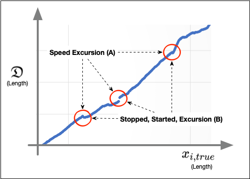
**Figure 2:** Tool behavior is recorded in the drift.

Figure 2 is a representative plot of relative bias using the methodology of Champlin 2025^[1]. This figure shows the combined bias accumulation of a recent inline inspection, labeled as (B), and an older, reference inspection, labeled as (A).

Three points of non-linear behavior are circled. The left and right points are sharp corners, and the center point is a discontinuity. In this example, the inspection vendor called out aberrant inspection tool behavior in both inspections at all three circled locations. All three circled locations were called out as speed excursions in Inspection $(A)$ and as a tool stoppage, followed by a restart, followed by a speed excursion in Inspection (B).

In the smooth region to the left of the first point, there were no called-out aberrant tool behaviors. In the rougher region to the right of the left-most point, there were many tool stops, starts, and speed excursions in Inspection (B).

In this example, a correlation appears to exist between roughness in the relative bias and aberrant tool behavior. I don’t have enough inspection data to determine if this is a real correlation or just a coincidence, as it seems to hold true for the datasets I have examined.

What I CAN draw from this, however, is my hypothesis as to where these signals in the bias originate. This (for now) speculation helps explain why odometry readings disagree and cannot be compared directly. Proceed to the last section for the punchline.

C. L. Champlin, Using odometry drift to match ILI joint boundaries for run comparisons, International Journal of Pressure Vessels and Pipelines, Vol. 213, 2025. ↩︎

Summing up – explaining weird odometry behavior

The state machine model can explain patterns in the relative odometry bias as a consequence of secondary pig motion inadvertently embedded into the odometry signal. Consider how changes in the forces acting on a pig might affect these values. These forces, whether from changes in fluid speed or a new vibration from a corroded pipe wall, will be detected by the IMUs and wheels tracking the pig motion, and encoded into the position estimates. This will create small fluctuations in the rate of error accumulation of the odometry estimate.

Although these nuanced measurements cannot be observed directly in the odometry of a single inspection, they may be seen indirectly in the relative bias measurement, which is a linear combination of two sets of odometry values.

Many interesting inspection phenomena can be correlated to patterns in the drift. Stopped pigs appear as discontinuities. Rough drift signals can correlate to severe generalized internal corrosion. Joint replacements can sometimes be identified by the drift dropping, where the tool sped through the new pipe, and rising, where the tool slowed through the original pipe.

Although there has been no formal study, this state-machine model of odometry differences can nicely explain these phenomena.

Conclusions

The traditional explanation that “wheel slip” is the cause of odometry discrepancies would imply that odometry would always under-report the length of a pipeline segment. This is not what happens in practice.
Experienced practitioners will attest that odometry errors can both increase and decrease the apparent length of an inspection. This observation is consistent with the new model presented here.
Odometry readings are unique to each tool and cannot be compared due to the tiny physical and electrical differences between them. These discrepancies cause subtle differences in how bias accumulates, resulting in each tool having its own unique odometry signature. The pattern of odometry values generated by a particular tool is behavior that emerges from its unique microscopic properties and the environment in the pipe at the time of the inspection.

Why can’t I use odometry for ILI runcoms?

Introduction

Table of Contents