Overview
Undergraduate engineering students at the Colorado School of Mines must participate in a two-semester, multidisciplinary capstone project. These projects are intended to allow the students to apply what they have learned in the classroom to a real project. Our goal for this project was to build an integrated cleaning and inspecting pig (ICIP). These inexpensive tools can be used to monitor an operating pipeline.
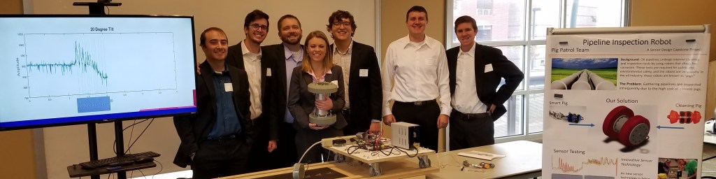
We were proud that our efforts were judged the “Best in Show” by a panel of industry experts at the capstone design showcase at the end of the year-long project.
This article has two parts. In this first half, I describe the tool and our design choices. In the second half, I run through a rough probability of detection (POD) calculation for our pig.
For this project, I was the customer. The 7-member team consisted of six mechanical engineering students and one engineering physics student. The students were: Project Manager: Logan Nichols, Technical Lead: Evan Marshall, Comm. Lead: Grant Deshazer, Team Members: Matthew Atherton, Victoria Steffens, Kyle Crews, Evan Thomas.
This project happened a while ago. I am getting caught up over the holidays.
The contents of the post are:
Project Summary

This project aims to build an inexpensive screening pig that can supply a pipe operator with insight into the state of the pipe when high-resolution tools are unavailable. This would be between or instead of full inspections. The use case is that this screening tool will be run frequently, and a composite understanding of the pipe wall will emerge by combining multiple assessments. To that end, the pig should be easy to operate and repair. A field hand should be able to offload data and prepare the pig to be rerun every two weeks.
Specifications and budget
The tables below are the mechanical specifications of the 8″ pig prototype we built. Capabilities followed by 3 stars (***) are based on theoretical calculations and require more testing.
| Specification | Value |
|---|---|
| Front disk diameter | 8.5 in |
| Rear disk diameter | 8.0 in |
| Total length | 11.0 in |
| Mandrel length | 6.5 in |
| Disk urethane density | 4.4‐4.7 lbs/ft^3 |
| Min turn radius*** | 12 in (1.5D) |
| Capability | Value |
|---|---|
| Number of sensors | 15 |
| Nominal sensor offset from wall | 0.25 in |
| Smallest depth | 3/32 in |
| Max sensor angle | 20 deg |
| Battery life*** | 5 hrs |
| Sample rate*** | 500kHz to 1MHz |
| Max velocity*** | > 75 mph |
The assumptions behind each of these values are in the text that follows.
Total project expenditures: $870
Since our supplier only had 3-sensors available for us to purchase and since our proof of concept was implemented in aluminum instead of steel, the cost of a working prototype will be higher.
Estimated cost of prototype: $3,000
Design Choices
Sensor selection
The choice of sensor is the primary driver of the mechanical design. In addition to the desire to detect internal and external defects, we imposed two usage-based constraints that, in turn, further restrict our choice of sensor. First, a solo worker must be able to maneuver the 8″ pig into and out of the pipe. This implies that the pig must weigh less than 50 pounds. This rules out heavy sensors like MFL. Second, the pig must be short enough to negotiate a 1.5D curve. This rules out the selection of long sensors like remote-field eddy current. Another consideration is that sensors with a large current draw need bigger batteries. This increases cost and weight and shortens run time. Low current draw, then, became an important criterion. Finally, commercial availability becomes an important criterion since we want to keep the costs down.
After considering a wide range of sensor types, most of which we could reject with simple thought experiments, we focused on three sensor candidates – eddy current (EC), electromagnetic acoustic transduction (EMAT), and inductive proximity sensors. We did detailed studies of each of these types.
Although they can only detect internal corrosion, EC sensors are attractive because they are inexpensive and adaptable. However, we ruled them out for this project because we were concerned that testing the many possible permutations of transmitting and receiving coil would distract us from our goal of creating a working pig.
We wanted to get EMAT sensors to work since they would give us visibility to the inner and outer pipe walls. Unfortunately, EMAT is a very sensitive sensor design. It requires small stand-off distances that we were concerned we could not maintain with a coarse tool like ours. Further, the circuitry for these sensors is complex and requires plenty of electric current to induce acoustic signals in the pipe wall. We felt that using these sensors would distract us from our goal of creating a working pig.
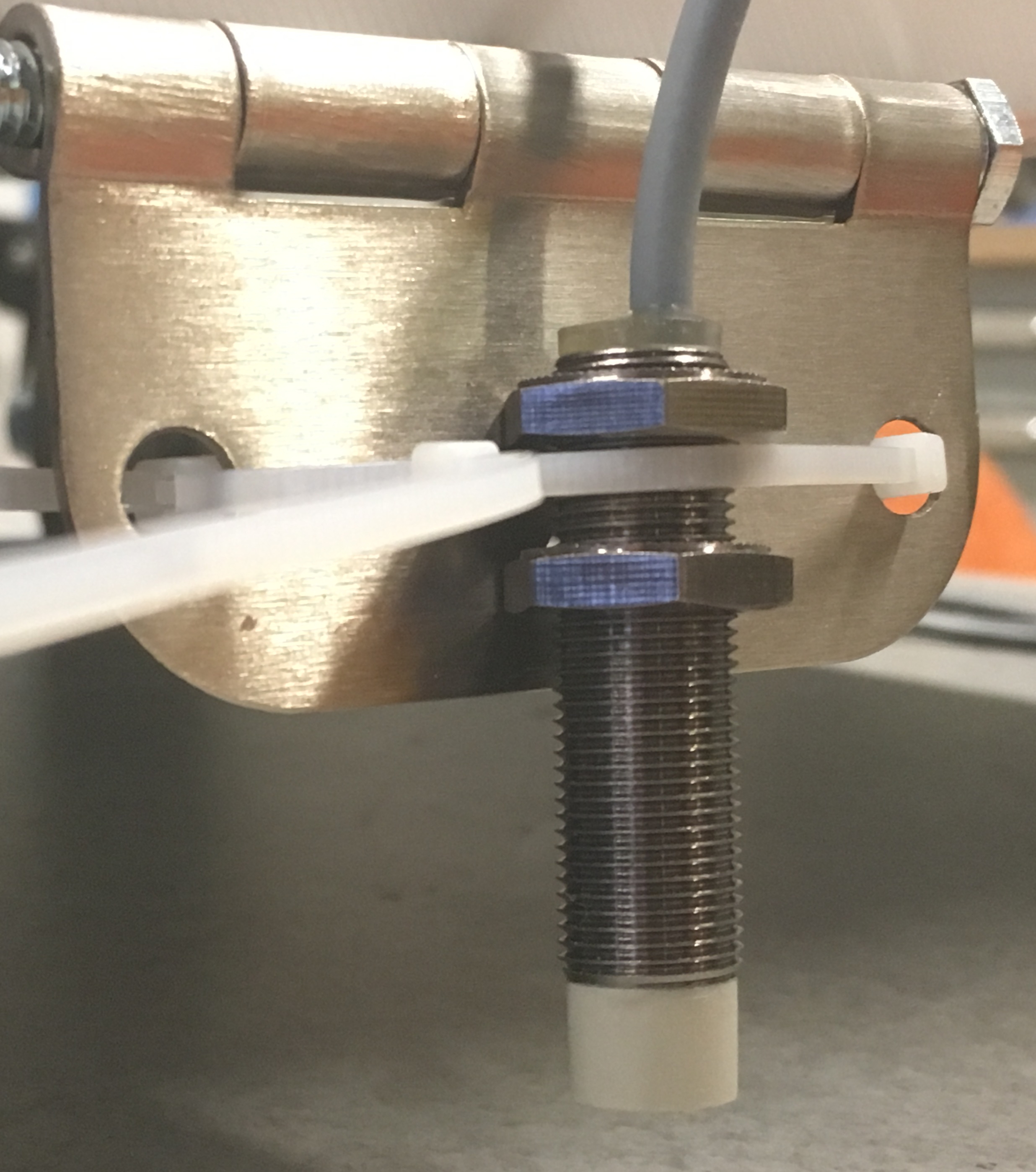
In contrast to EC and EMAT, inductive proximity sensors are commonly used in manufacturing and thus are inexpensive and widely available. They operate on the same principle as EC sensors but use a single inductive coil for both transmitting and receiving. This simple oscillating magnetic field outputs a voltage proportional to distance, making the circuitry easy to build and the signal easy to interpret. Further, this single coil design reduces the current draw, reducing our dependence on expensive and heavy batteries. Additional advantages include their ruggedness and insensitivity to surface contaminants. Finally, inductive proximity sensors have a perfect operating range of up to an inch and a half.
There are two main drawbacks to inductive proximity sensors. First, like an eddy current sensor, inductive proximity sensors are primarily useful for internal defects and are blind to external ones. Their ability to penetrate metal falls off with the square of the distance. Second, they are not effective for non-ferrous pipes. A complete solution for pipes made from multiple pipe wall materials will require other pigs with other sensors.
In later sections, we demonstrate through experimentation that inductive proximity sensors are an excellent choice for this application. They give us a reasonable resolution of 3/32 inches in corrosion feature depth. Our radial resolution is constrained by the packaging of the sensors we bought to 1/2 inch. This could well be improved with custom packaging. Our axial resolution is determined by traversal speed. Since these simple sensors can operate at high sample rates with minimal increase in current draw, our pig should be able to make Nyquist-theoretic continuous scan velocities over 75 mph. Because we are operating well inside the maximum range for these sensors, we found a maximum deflection angle of 20 degrees. This means the sensors can be fouled by a significant amount of gunk and still take valid readings.
The sensors we selected were from Fargo Controls, inc. We picked their Long Range Inductive Proximity Sensor X0036 based purely on its specifications. Before going into production, it would be nice to do a comparative study of other similar sensors.
Mechanical package
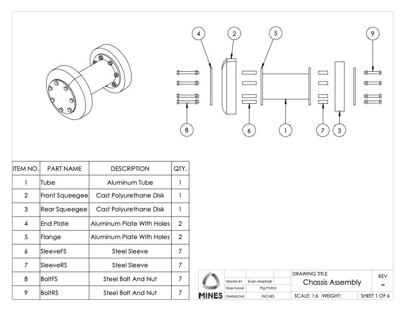
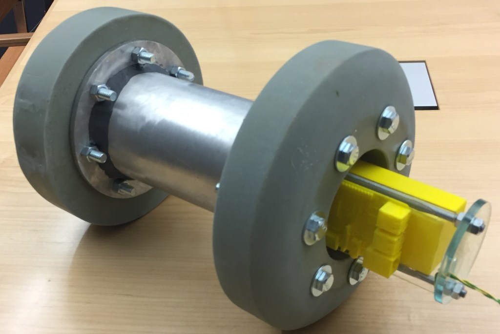
The picture above shows the final proof-of-concept mechanical package based on a mandrel-cleaning pig. Referring now to the “chassis assembly” drawing sheet. The pig length, excluding the thickness of the bolt heads ⑧ and ⑨ and including the lengths ④+②+①+③+④, is 11.0 inches. The central mandrel ① is 6.5 inches long. The mandrel’s outer diameter is 4.1 inches, and its inner diameter is 3.75 inches. The front drive disk ② is 2.5 inches long and 8.5 inches in diameter. The rear, sensing and stabilizing disk ③ is 1.5 inches long and 8.0 inches in diameter. The plates ④ secure the disks to the mandrel. Not shown in this drawing is a 3.0-inch circular bulkhead in the front plate, which allows access to the electronics package.
The electronics package within a sliding frame is sealed into the mandrel body. The lid of this chamber is sealed with a circular bulkhead. This bulkhead is made of transparent material in the photograph above. In a functioning device, this would be constructed of steel and designed to seal against the prescribed operating pressure.
The shape of the cast polyurethane disks was dictated mainly by the cake pan we used as a mold. The larger diameter of the front disk is designed to seal against the pipe’s inner wall and pull the pig forward. The rear disk is smaller to reduce mechanical chatter from friction with the pipe wall. The proximity sensors are embedded in the urethane of these rear disks. The wires include strain relief to allow the sensors to move as the disk flexes during pig transit.
Electronics package

The “Electronics Assembly” drawing above shows the mechanical packaging of the electronic components in the electronics bay of the pig’s mandrel, which is called the “tube” in the mechanical drawing of the previous section. The electronic components are secured to the platform ③ between two pressure-sealed bulkheads ① in the mandrel. The electronics are designed around a single-board computer called a Raspberry Pi ⑤.
An Arduino microcontroller is mechanically attached to the header pins on the single-board computer in a “shield” configuration. The wires from the sensors embedded in the trailing disk enter the electronics bay through pressure and explosion-safe connectors. Leads from these connectors are affixed to the microcontroller by quick-connects.
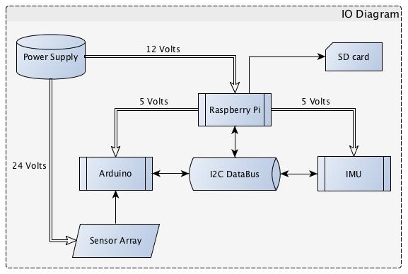
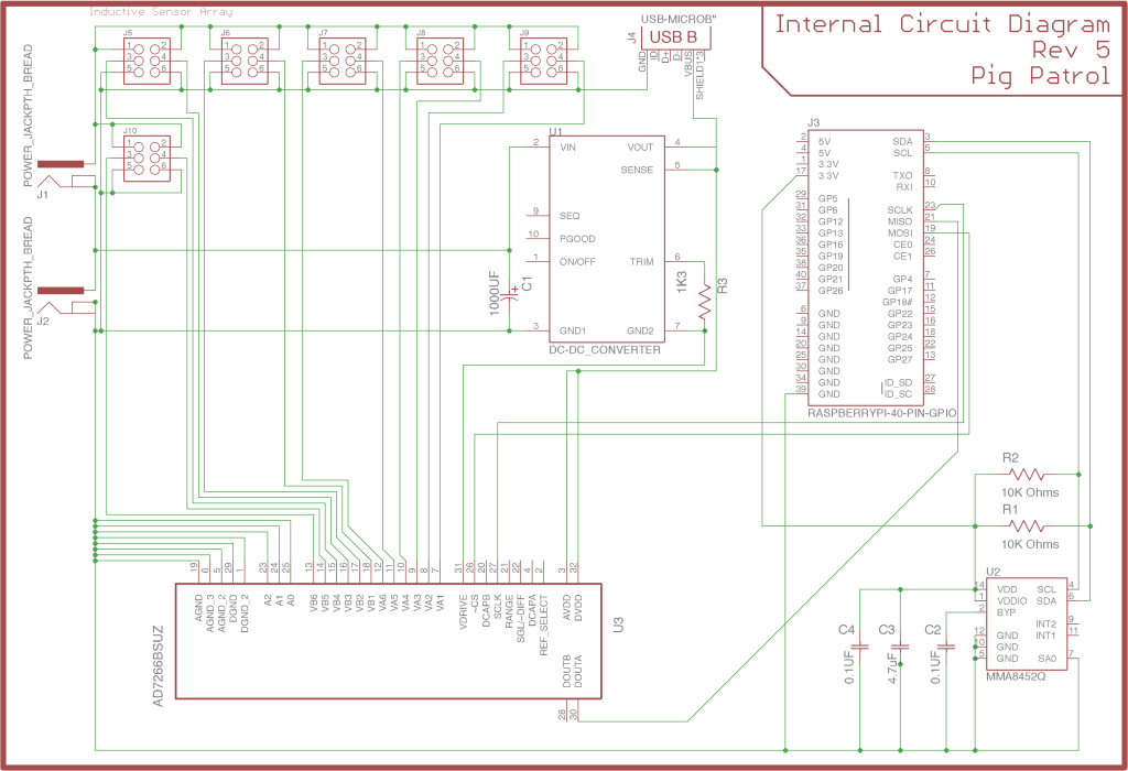
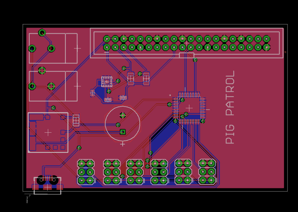
The image carousel above contains four diagrams illustrating the logical relationships between the electronic components. The images in this carousel are the “I/O Diagram,” the “Data Collection Sequence” diagram, the logical “Internal Circuit Diagram,” and finally, a circuit board design labeled “Pig Patrol” for an analog-to-digital converter that would replace the Arduino microcontroller.
The “I/O Diagram” shows the power distribution from the onboard 24-volt battery to the physical elements (double-stroke arrows) and the logical information flow between these elements (single-stroke arrows). The Raspberry Pi single-board computer is the foundation for this arrangement. It distributes power to the Arduino microcontroller, the inertial measurement unit (IMU), and the wheel encoders (not shown). Its I2C data bus provides a high-speed universal connection between the sensing elements and the SD card, providing nonvolatile data storage.
The “Data Collection Sequence” is a swim-lane diagram showing the events’ interaction between the Raspberry Pi single-board computer (SBC), the Arduino microcontroller, and the inductive sensors. The SBC contains an accurate clock with a high clock rate that triggers data reads from the sensor array. At each cycle interval, the SBC sends a read request to the microcontroller, which polls the sensors for their current values and stores them in a byte array of voltage readings. This array is transmitted across the i2C bus and converted into an array of short bytes for efficient storage in the SD card.
The “Internal Circuit Diagram” shows a forward-looking circuit intended to replace the Arduino microcontroller with a serial analog-to-digital converter to achieve much higher data sample rates. A custom PCB design for this faster circuitry is the final image in the carousel. This newer circuit would replace the Arduino shield and would provide a secure home for the IMU. This custom board would plug directly into the Raspberry Pi’s header, providing short data pathways and mechanical stability.
Preview of the next installment
The next installment of this write-up characterizes the sensors. It uses the sensor signals to estimate the axial resolution, the radial resolution, and the sensitivity of the sensors to various defects.

Leave a comment