The most common GCS distance calculation, the Spherical Law of Cosines (SLoC), gives poor results at short distances. This is an issue when calculating joint lengths using latitude/ longitude pairs. These distances are typically between 20 and 60 feet (6 and 18 meters). At these short distances, the spherical law of cosines has a precision of only 4.5% in my high-latitude test data set. This is about 2 feet of error every 40 feet (0.6 m in 12 m). In contrast, the three alternate techniques I compare with the SLoC all find short-segment lengths with a precision of 0.05%. This is about 1/4 inch over 40 feet (0.6 cm in 12 m). An improvement of 2 orders of magnitude!

Here I will demonstrate three alternative small-distance calculations and how to implement them in Excel. I will show a flat earth approximation, an angle-difference modified spherical law of cosines, and the haversine calculation. After giving a brief overview of the theory behind all four of these calculations, I present the test data set and a table that compares the normalized error for all four methods’ distance calculations on that data set. After this, I provide tables showing the structure and key formulas from the spreadsheet. Finally, after giving a link to a downloadable copy of an Excel spreadsheet with working implementations of all four methods, I have included a table with all the GIS points used and the lengths of the segments between them as calculated by the GeoPy library.

Key concepts

Many people know that latitude and longitude pairs describe points on the grid of a spherical coordinate system. They can represent any location on the earth. Longitude is the x-coordinate, and latitude is the y-coordinate. There are many nuances. The Wikipedia entry for geographic coordinate systems provides a sense of the complexities. At issue are measurement units, points of origin, and models for the earth’s shape.

The current discussion addresses the trigonometry of this spherical coordinate system. Points in this curved space are specified by a triple where is the length of a vector anchored at the center of the sphere. The angle in the horizontal plane, , is the longitude. It is analogous to the x-coordinate in a Cartesian grid. The angle describing the vertical displacement, , is the latitude. It is an analog to the y-coordinate.

With this system, the distance between any two points on the sphere, such as points and in the figure, is simply the arc length of the shortest sector of a great circle that passes through them. In this case, the distance is simply the arc length in radians times the radius of the sphere, .

The challenge addressed in the rest of this document is to find the angle . Because we are concerned with short distances, this angle is extremely small.

For this discussion, we will model the earth as having a constant radius. According to the NASA Earth Fact Sheet, the earth’s mean radius is , which is . If you are interested, this article by the Math Doctors discusses some nuances about the selection of R.

Flat earth approximation

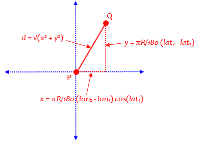
The flat earth approximation says that when the distance is small, a cartesian grid around the point pair is uniform. That is to say, the curvature is insignificant over short distances.

One must convert from angle to distance to represent distance on this grid. Since all lines of latitude are great circles, the conversion from angle to length for the y-axis is trivial. As shown in the Key concepts section, the vertical grid spacing is simply . In the figure, for a specific distance, the angle is the difference between the latitudes, . The factor is used to convert from degrees to radians. Since this value is dimensionless, the units of are the same as those used for .

The spacing on the x-axis is more complicated. Notice that the size of the horizontal circle, representing longitude, gets smaller with increasing latitude, vanishing completely at the poles. The consequence is that the distance represented by each degree of longitude on the x-axis decreases with the distance from the equator. The radius must be reduced by the cosine of the latitude so that the horizontal grid spacing is . Thus for a specific pair of points, the x-component of distance is .

Finally the Manhattan distance is converted to the Euclidean distance by .

For a deeper discussion of this topic see this article by the Math Doctors.

Law of cosines

In Euclidean geometry, the law of cosines is a consequence of the dot product. It says that given the length of two sides of a triangle and the angle between them, one can find the length of the side opposite the angle. In the planar figure on the right, given the lengths of sides , and , and the angle , one can find the length of side as .

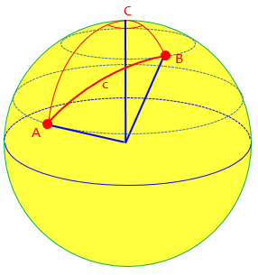
This formulation is typically adapted to spherical coordinates by picking a pole (north or south, depending on the hemisphere) as the third point. This would be analogous to the point with corresponding angle in the figure on the right. This gives us the spherical triangle shown in the figure on the left. Here points and are the points we are trying to find the distance between, and point is the pole. Then the known distances and can be found as as above.

This formulation is called the Spherical Law of Cosines and it is given for radians as

.

A quick internet search will find many examples of this formulation and this result. A clear example is this article at Wolfram Mathworld.

At short distances the included angle is very small. The values of cosine approach 1 slowly. As an example,

and

.

The inverse cosine has a difficult time returning the correct angle since these values are all so close. Because of this, the spherical law of cosines has poor performance at small distances.

The Math Doctors applied the angle-difference identity to the standard Spherical Law of Cosines formulation and arrived at this subtly different result:

While apparently not their intent, this variant seems much better behaved at small distances. I compare both of these variants in my analysis below.

Haversine distance calculation

The Geographic Information Systems usenet FAQ archive gives several formulas for distance measures. It claims that the haversine calculation yields “mathematically and computationally exact results.” It points to a 1984 paper by R.W. Sinnott, “Virtues of the Haversine” in Sky and Telescope, vol 68, no. 2, 184, p.159.

According to an article by the math doctors a “haversine” is “the name of one of several lesser-known trigonometric functions that were once familiar to navigators and the like. The VERSINE (or versed sine) of angle A is . The HAVERSINE is half the versine, or . With a little math, you can show that hav(A) = (1-\cos(A))/2 = \sin^2(A/2).”

The original formulation relies on a min(a,b) function to avoid singularities. Unfortunately, this approach relies on the practitioner to track each point’s quadrant to correctly evaluate the function. A more programmer-friendly approach is to use the arctan2 function, which returns the correct quadrant and gracefully handles the poor conditioning of the cosine function near zero.

Allowing the math doctors to cover the details in their article the final formulation as manifested in my Python implementation is

R = 6371e3 * 3.28084 # meters x feet / meter = feet

# conversion function
def deg2rad(deg) :
    return deg * math.pi/180

# geodistance using the haversine formula
def hDist(lat2, long2, lat1, long1) :
    dLat = deg2rad(lat2 - lat1) 
    dLong = deg2rad(long2 - long1)
    
    a = math.sin(dLat/2)*math.sin(dLat/2) \
        + math.cos(deg2rad(lat2)) * math.cos(deg2rad(lat1)) \
        * math.sin(dLong/2) * math.sin(dLong/2)
    
    c = 2 * math.atan2(math.sqrt(a),math.sqrt(1-a))
    
    return R * c # distance in units of R (feet here)

Experimental Setup

To compare the four methods’ ability to correctly estimate small distances I selected a location with a high latitude where errors in longitude would be the greatest. The location shown above is an open area near the University of Calgary campus. I picked vertices in a zig-zag pattern that would be easy to evaluate with the ruler tool. Also, I was interested in a range of segment lengths and orientations in the event that bearing has an impact on calculating results. The shortest segment in this set is 17.4 feet (5.3 meters). The longest segment is 50.7 feet (15.5 meters). The mean length is 32.5 feet (9.9 meters), with a median length of 32.3 feet (9.8 meters). While I tried to get a mix of orientations, most segments are nearly parallel to the equator.

General Approach

I used named ranges for each column. This approach invokes volatile functions in Excel which behave like vector functions in other languages like MatLab, R, and Python.

As presented here, the latitude and longitude values are expected as decimal values over the range [-180.180]. If your values are in degrees, minutes, seconds or have NSEW suffixes, they need to be converted. There are plenty of resources for these conversions. The Federal Communications Commission (FCC) offers a converter widget, and Microsoft provides a tutorial on how to do it in Excel.

Summary of Results

I used the GeoPy library to determine the ground truth length for each segment. This library uses a variable radius representing the shape of the earth as a flattened ellipsoid per the WGS-84 standard. I calculated the mean and standard deviation of the normalized error for each distance measurement approach described above. The table below shows a summary.

Implementation Details

The full spreadsheet may be downloaded here. This section describes the named ranges and the formula used for each approach as seen in this spreadsheet.

Flat Earth

This approach will become less precise as distances between points increase.

Spherical Law of Cosines

The first six (6) columns from the previous calculation plus the one column below.

The gpDist column is the same as the previous calculation.

This approach produces poor results at the small distances used for this analysis. As I understand from the literature, this approach performs well at larger distances.

Adjusted Spherical Law of Cosines

The first six (6) columns from the first calculation plus the one column below.

This approach works well at these distances. It is not clear how it will perform at larger distances. I did not test this.

Haversine Formula

The first six (6) columns from the first calculation plus the three columns below.

This approach was designed for large distances. It works well at small distances.

Conclusions

• All of the calculations are similar in complexity
• The haversine calculation produces good results at all scales, this is probably the best general choice
• Perhaps law of cosines is so common in the literature because it is easy to explain? It was the only approach that didn’t work at this scale
• It is intuitive that flat earth calculations would perform well, but the adjustment for latitude is important
• The spherical earth assumption seems to hold at these distances.
• I do not have an intuition for why the adjusted SLoC works. Any thoughts?

Resources

Movable Type Scripts : Calculate distance, bearing and more between Latitude/Longitude points
https://www.movable-type.co.uk/scripts/latlong.html

Math Doctors: Distances on Earth 2: The Haversine Formula
https://www.themathdoctors.org/distances-on-earth-2-the-haversine-formula/

FAQs.org: Geographic Information Systems FAQ
http://www.faqs.org/faqs/geography/infosystems-faq/

Wolfram MathWorld: Spherical Trigonometry
https://mathworld.wolfram.com/SphericalTrigonometry.html

Microsoft Support: ATAN2 function
https://support.microsoft.com/en-us/office/atan2-function-c04592ab-b9e3-4908-b428-c96b3a565033

Power-User: Why you should name ranges in Excel, and how to do it
https://www.powerusersoftwares.com/post/2017/05/27/why-you-should-name-ranges-in-excel-and-how-to-do-it

GeoPy Documentation: Calculating Distance
https://geopy.readthedocs.io/en/stable/#module-geopy.distance

Data Used